ML and AI Theory Seminar | University of California, Berkeley
Posterior Contraction Rates for Matérn
Gaussian Processes on Riemannian Manifolds
Viacheslav (Slava) Borovitskiy
https://vab.im

Posterior contraction rates
Beyond rates
Summary
Gaussian processes — random functions with jointly Gaussian marginals.
Determined by a mean and a kernel (covariance function).
Bayesian learning: prior GP + data = posterior GP
For zero prior mean and Gaussian noise of variance $\sigma_{\eps}^2$:
Probabilistic models: input ⟶ distribution (prediction + uncertainty)
Allows computing queries like probability of improvement: $\!\alpha(x) \!=\! \mathbb{P} \! \del{f(x) \!>\!\! f^*}$
They can drive selection of the next point to evaluate [Bayesian optimization]
Matérn kernels:
$$ \footnotesize k_{\nu, \kappa, \sigma_f^2}(x,x') = \sigma_f^2 \frac{2^{1-\nu}}{\Gamma(\nu)} \del{\sqrt{2\nu} \frac{\abs{x-x'}}{\kappa}}^\nu K_\nu \del{\sqrt{2\nu} \frac{\abs{x-x'}}{\kappa}} $$
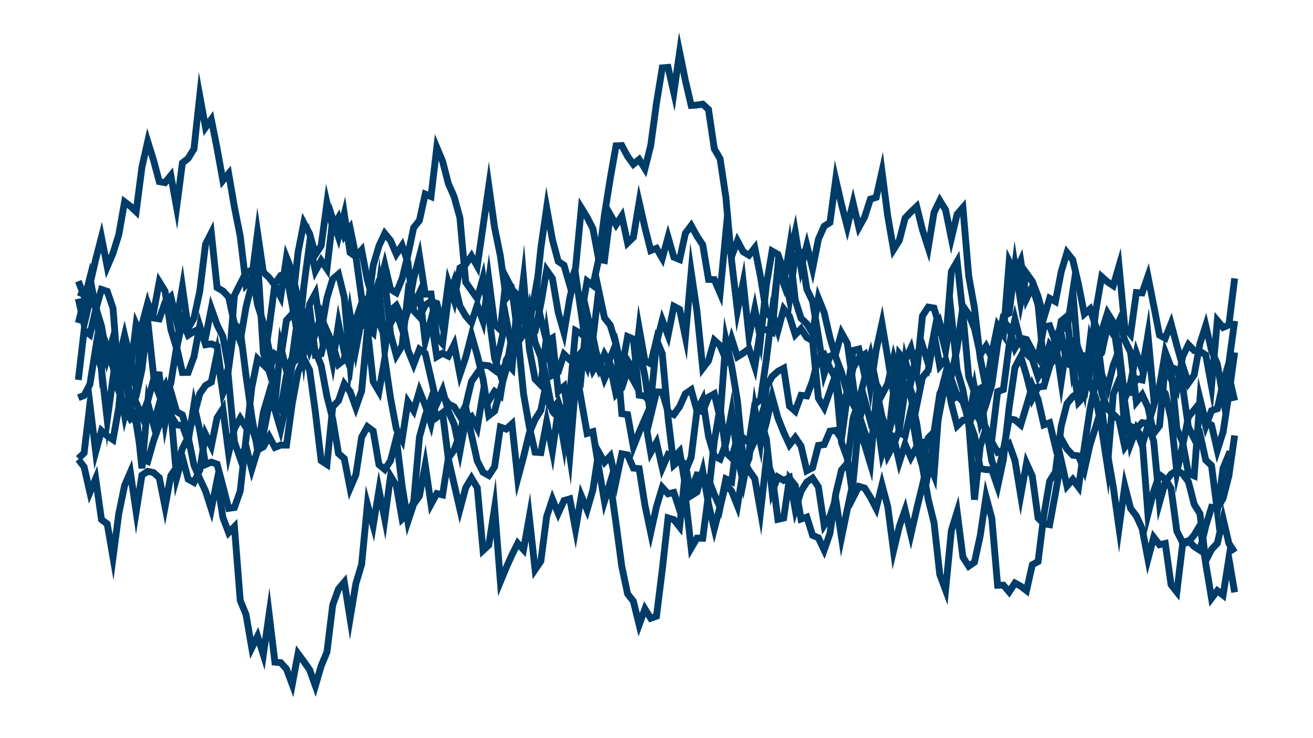
$\nu = 1/2$
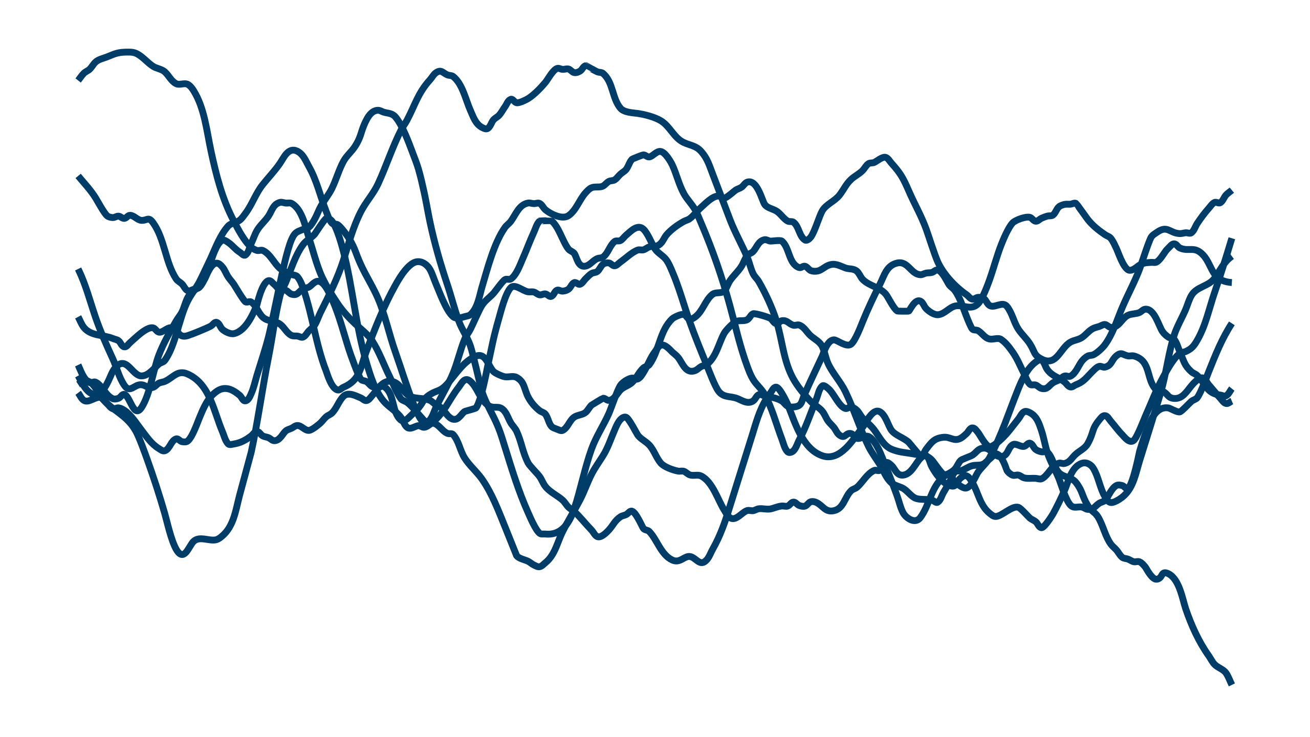
$\nu = 3/2$
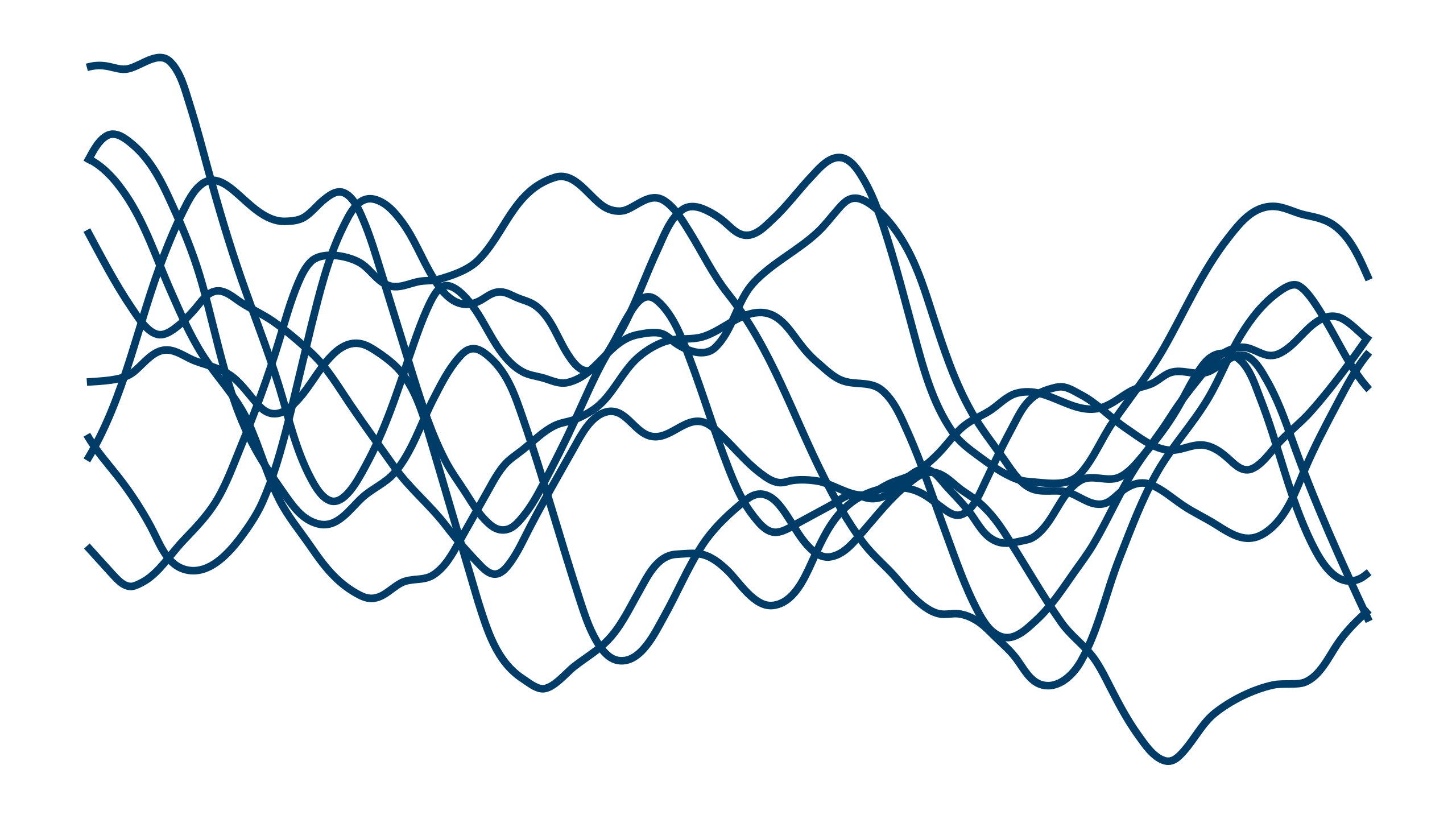
$\nu = 5/2$
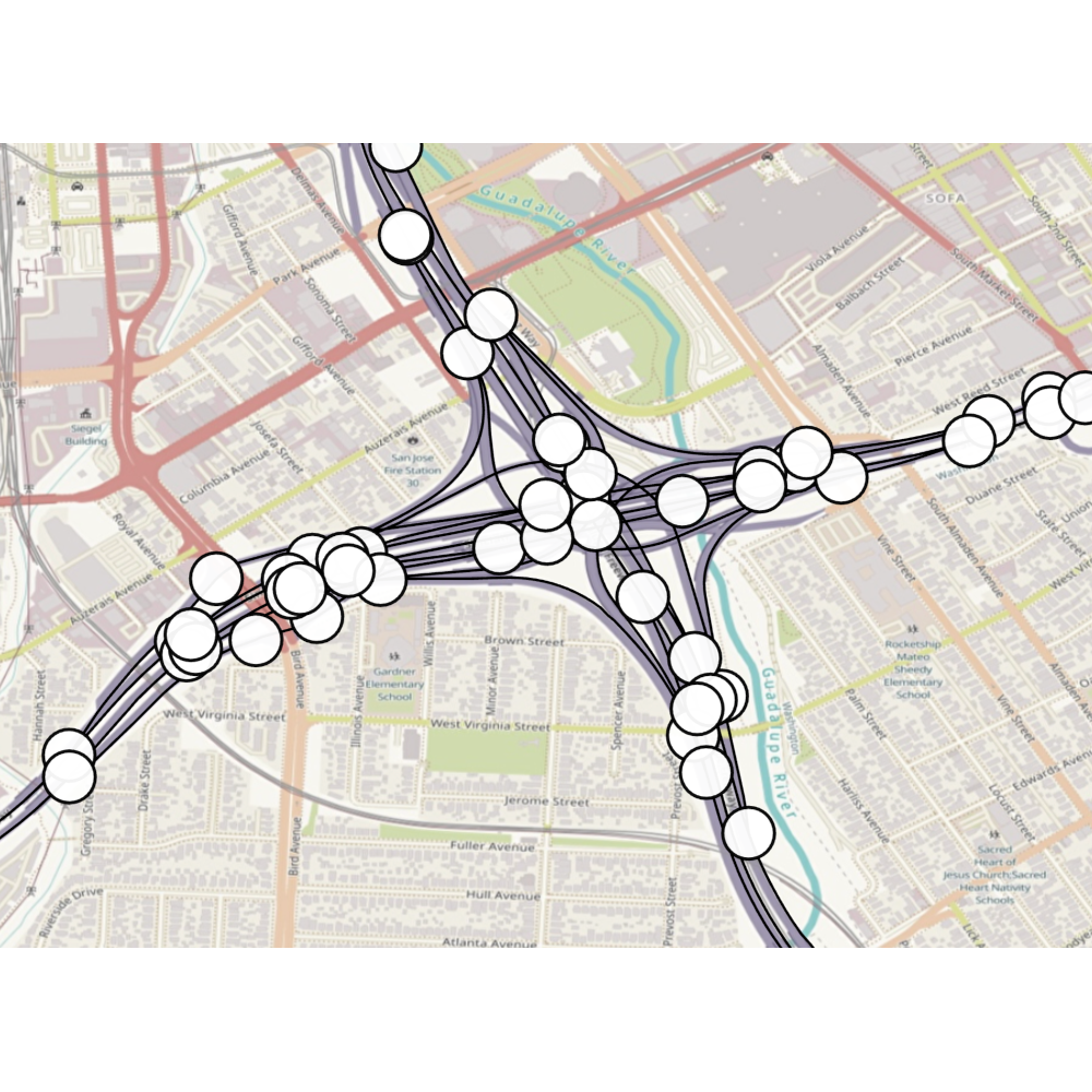
Geometric GPs: models defined on such domains that respect their structure.
In the squared exponential kernel, use the geodesic distance:
Not positive semi-definite for some $\kappa$.
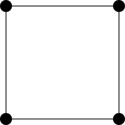
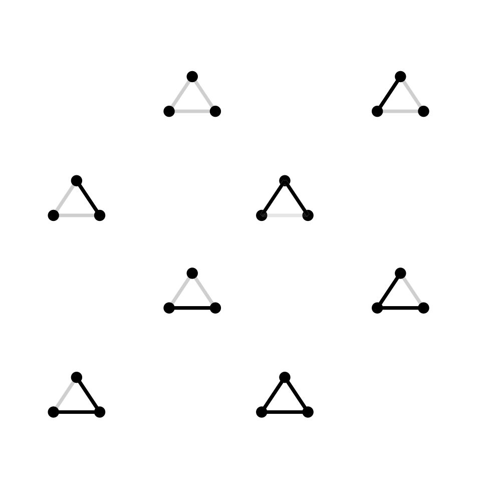
Graphs, unless isometrically
embeddable into a Hilbert space.
Schoenberg (Trans. Am. Math. Soc. 1938)
Manifolds, unless
isometric to $\R^d$.
Feragen et al. (CVPR 2015), Da Costa et al. (SIMODS 2025)
$$ \htmlData{class=fragment,fragment-index=0}{ \ubr{\del{\frac{2\nu}{\kappa^2} - \Delta}^{\frac{\nu}{2}+\frac{d}{4}} f = \c{W}}{\t{Matérn}} } $$
Whittle (Bull. Internat. Statist. Inst 1963)
Lindgren et al. (JRSSB 2011)
Intrinsic Matérn prior, through its Karhunen–Loève expansion:
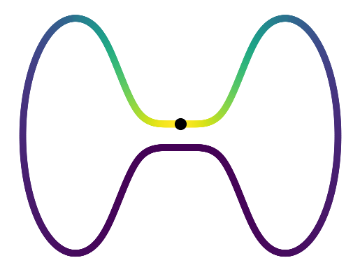
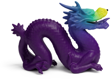
Matérn kernels $k(\bullet, x)$
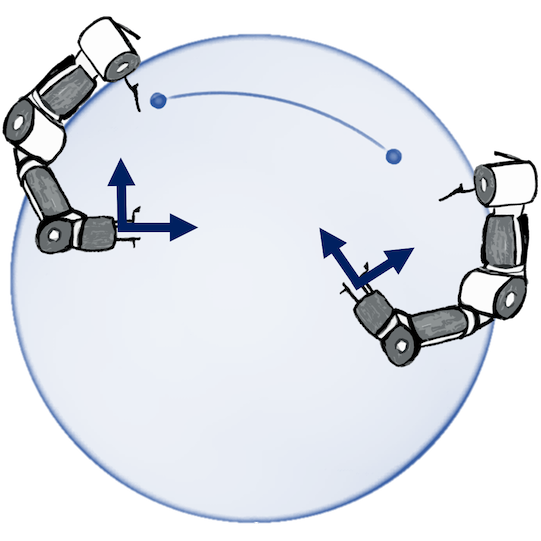
Robotics
Learn the orientation of a robotic arm
with less data than baselines.
Jaquier et al. (CoRL 2022)
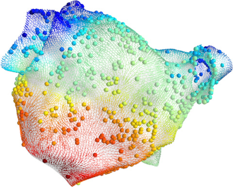
Medicine
Regression on a manifold which models
the geometry of a human heart.
Coveney et al. (Phil. Trans. A 2020)
$\c{M} \subset \R^D$, isometrically embedded.
Take the ordinary Matérn kernel, with the Euclidean distance $\norm{x - x'}_{\R^D}$,
and restrict it to $x, x' \in \c{M}$. This is the extrinsic Matérn prior.
Intrinsic
Formulated directly on the manifold.
Need to know $\c{M}$.
Extrinsic
Agnostic to the manifold geometry.
Works even when $\c{M}$ is unknown.
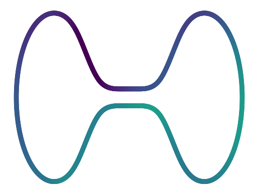
Intrinsic
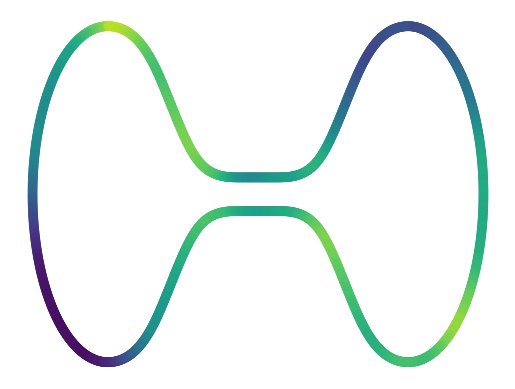
Extrinsic
Close in the ambient space,
far along the manifold:
spurious dependencies.
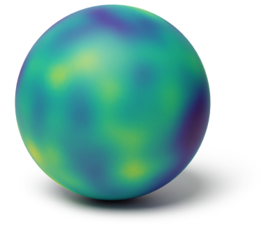
Intrinsic
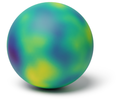
Extrinsic
Distances are approximated well:
little qualitative difference.
Wouldn't it be great to have a proof
that intrinsic models are better than ambient ones?
I met Paul Rosa, working on the same question, hence the paper:
(PhD student at Oxford at the time, now a postdoc in Cambridge)
Truth
Model
Does the posterior uncover $f_0$ as $n \to \infty$? How fast?
By Jensen's inequality, the posterior mean $m_{\text{post}}$ inherits the rate.
$f$: Matérn prior on $[0, 1]^d$, with smoothness $\nu > d/2$.
$f_0 \in H^\beta \cap \mathrm{C}\mathrm{H}^\beta$ (Sobolev and Hölder), with $\beta > d/2$.
Best when true and prior smoothness match, $\nu = \beta$: $\;n^{-\frac{2 \beta}{2 \beta + d}}$
Minimax: no estimator does better uniformly over a smoothness class.
$\h{f}$: any estimator, a rule mapping data to functions. $\;\c{F}_\beta$: a ball in $H^\beta \cap \mathrm{C}\mathrm{H}^\beta$.
The posterior mean attains this at $\nu = \beta$: $C$ depends only on norms of $f_0$.
Sobolev space $H^s(\c{M})$: decay of Laplace–Beltrami coefficients.
Besov space $B_{\infty, \infty}^s(\c{M})$: Hölder-like, via approximation by low frequencies.
$P_j$: smooth low-pass filter, keeps $\sqrt{\lambda_l} \leq 2^j$ and removes $\sqrt{\lambda_l} \geq 2^{j + 1}$.
$f$: intrinsic Matérn prior with smoothness $\nu > d/2$.
$f_0 \in H^\beta(\c{M}) \cap B_{\infty, \infty}^\beta(\c{M})$ with $\beta > d/2$.
Minimax optimal at $\nu = \beta$, with the intrinsic dimension $d$.
Yay!
Gaussian prior with continuous sample paths and RKHS $\bb{H}$:
If $\;\varphi_{f_0}(\eps_n) \leq n \eps_n^2$, the posterior contracts at the input locations:
Holds for every fixed $\v{x}$, with the same constant.
The covariance operator is diagonal in the $f_j$,
with eigenvalues $\asymp (1 + \lambda_j)^{-(\nu + d/2)}$.
So $\bb{H} = H^{\nu + d/2}(\c{M})$, with equivalent norms.
The length scale $\kappa$ only changes the constants.
Small ball probabilities are governed by the entropy of the RKHS unit ball:
$N(\eps)$: number of uniform $\eps$-balls needed to cover the unit ball of $\bb{H}$.
By step 1, the unit ball of $\bb{H}$ lies in a Sobolev ball on $\c{M}$.
Charts reduce the entropy of that ball to the known bound on $\R^d$.
We need $g \in \bb{H}$ uniformly $\eps$-close to $f_0$, with a small RKHS norm.
$f_0$ itself need not lie in $\bb{H} = H^{\nu + d/2}(\c{M})$: it may be too rough.
Instead, keep only its low frequencies: $\;g = P_j f_0 \in \bb{H}$.
Higher cutoff: smaller error
Because $f_0 \in B_{\infty, \infty}^\beta(\c{M})$.
Higher cutoff: larger norm
Because $f_0 \in H^\beta(\c{M})$, for $\nu \geq \beta$.
Taking $\;2^{-\beta j} \approx \eps\;$ gives $\;\norm{g}_{\bb{H}}^2 \lesssim \eps^{-\frac{2}{\beta} (\nu + \frac{d}{2} - \beta)}$.
For $\nu \geq \beta$, the decentering term dominates:
Solving $\;\varphi_{f_0}(\eps_n) \leq n \eps_n^2\;$ gives $\;\eps_n \propto n^{-\frac{\beta}{2 \nu + d}}$.
For $\beta > \nu$: also $f_0 \in H^\nu(\c{M}) \cap B_{\infty, \infty}^\nu(\c{M})$, so replace $\beta$ by $\nu$.
Altogether, $\;\eps_n \propto n^{-\frac{\min(\beta, \nu)}{2 \nu + d}}$.
From the input locations to $\;\norm{f - f_0}_{L^2(p_0)}$.
We follow van der Vaart and van Zanten (JMLR 2011, Theorem 2).
The main change: we must prove Hölder regularity of prior samples on $\c{M}$.
Otherwise, a rough $f$ could fit at the inputs and miss elsewhere.
Driscoll's theorem and Sobolev embedding only give $\gamma < \nu - d/2$.
Instead, we use Kolmogorov's criterion in charts.
The hard case is $\gamma > 1$, where it must be applied to derivatives of $f$.
The extrinsic process is completely agnostic to the manifold geometry.
We would expect it to be less performant.
A slower rate would be the proof we were hoping for.
$f$: extrinsic Matérn prior with smoothness $\nu > d/2$.
$f_0 \in H^\beta(\c{M}) \cap B_{\infty, \infty}^\beta(\c{M})$ with $\beta > d/2$.
The same rate. Yikes!
The dimension in the exponent is $d$. $D$ enters through the constant $C$.
The prior is not designed to be adaptive, but it adapts to the manifold.
Restriction
Ambient RKHS: $\tilde{\bb{H}} = H^{\nu + D/2}(\R^D)$,
with equivalent norms.
Trace and extension
Bounded linear maps, $\f{Tr} \o \f{Ex} = \f{id}$,
for $s > \frac{D - d}{2}$.
Restricting to $\c{M}$ loses $\frac{D - d}{2}$ of smoothness: $\;\nu + \frac{D}{2} - \frac{D - d}{2} = \nu + \frac{d}{2}$.
$\bb{H}$ is norm-equivalent to $H^{\nu + d/2}(\c{M})$, as for the intrinsic process!
Up to norm equivalence, the RKHS is determined by $\nu$ only.
So the rates do not see the length scale $\kappa$ either.
Similar in spirit to Yang and Dunson (Annals of Statistics 2016).
Extrinsic mixtures of squared exponential GPs: optimal rates for Hölder smoothness $\leq 2$.
In this setting, asymptotic rates cannot detect geometry.
Differences are down to constants. So we look at errors numerically.
$\tau = \mathrm{i}$: intrinsic. $\;\tau = \mathrm{e}$: extrinsic. $\;\bb{H}^{(\mathrm{i})}$: the intrinsic RKHS.
Inputs $\v{x}$ fixed, $\;\v{y} = f_0(\v{x}) + \v{\eps}$, with $\v{\eps}$ the noise.
A function of $t \in \c{M}$: shows how error varies across the manifold.
Posterior means are linear in the data, with weights:
Reproducing property, then supremum over the unit ball:
Intrinsic
Simply the posterior variance.
Extrinsic
Approximate the norm numerically,
on points sampled uniformly from $\c{M}$.
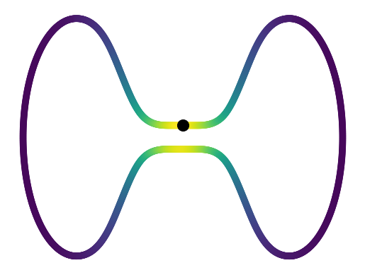
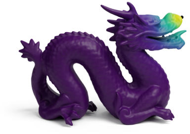
Intrinsic kernel
Extrinsic kernel
Intrinsic kernel
Extrinsic kernel



Mean of $v^{(\tau)}(t)$ over $t \in \c{M}$. Shading: spread over the 10 repetitions.
Dumbbell, dragon
Geometry differs from the ambient space.
Intrinsic: lower errors.
Sphere
No bottleneck-like areas.
Both models perform similarly.
The gap depends on the geometry, but the rates alone do not show it.