Talk at the Università della Svizzera italiana
Geometric
Gaussian Processes
Viacheslav Borovitskiy (Slava)


Definition. A Gaussian process is random function $f$ on a set $X$ such that for any $x_1,..,x_n \in X$, the vector $f(x_1),..,f(x_n)$ is multivariate Gaussian.
May refer to a random function / distribution, depending on the context.
Gaussian processes are characterized by
Notation: $f \~ \f{GP}(m, k)$.
The kernel $k$ must be positive (semi-)definite.
Takes
giving the posterior (conditional) Gaussian process $\f{GP}(\hat{m}, \hat{k})$.
The functions $\hat{m}$ and $\hat{k}$ may be explicitly expressed in terms of $m$ and $k$.
Goal: minimize unknown function $\phi$ in as few evaluations as possible.


Also
$$ \htmlData{fragment-index=0,class=fragment}{ x_0 } \qquad \htmlData{fragment-index=1,class=fragment}{ x_1 = x_0 + f(x_0)\Delta t } \qquad \htmlData{fragment-index=2,class=fragment}{ x_2 = x_1 + f(x_1)\Delta t } \qquad \htmlData{fragment-index=3,class=fragment}{ .. } $$
$$ x_0 \qquad x_1 = x_0 + f(x_0)\Delta t \qquad x_2 = x_1 + f(x_1)\Delta t \qquad .. $$
assume $f$ unknown, model $f$ as a GP.
$$ x_0 \qquad x_1 = x_0 + f(x_0)\Delta t \qquad x_2 = x_1 + f(x_1)\Delta t \qquad .. $$
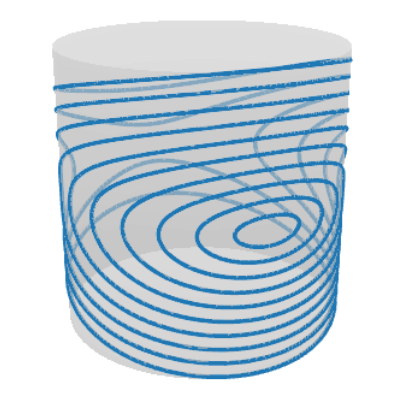

Phase portrait is periodic!
I.e. the state space is actually a cylinder!
Be able to: evaluate $k(x, x')$, differentiate it, sample $\mathrm{GP}(0, k)$.

$$
\htmlData{class=fragment fade-out,fragment-index=6}{
\footnotesize
\mathclap{
k_{\nu, \kappa, \sigma^2}(x,x') = \sigma^2 \frac{2^{1-\nu}}{\Gamma(\nu)} \del{\sqrt{2\nu} \frac{\abs{x-x'}}{\kappa}}^\nu K_\nu \del{\sqrt{2\nu} \frac{\abs{x-x'}}{\kappa}}
}
}
\htmlData{class=fragment d-print-none,fragment-index=6}{
\footnotesize
\mathclap{
k_{\infty, \kappa, \sigma^2}(x,x') = \sigma^2 \exp\del{-\frac{\abs{x-x'}^2}{2\kappa^2}}
}
}
$$
$\sigma^2$: variance
$\kappa$: length scale
$\nu$: smoothness
$\nu\to\infty$: RBF kernel (Gaussian, Heat, Diffusion)

$\nu = 1/2$

$\nu = 3/2$

$\nu = 5/2$

$\nu = \infty$
$$ k_{\infty, \kappa, \sigma^2}(x,x') = \sigma^2\exp\del{-\frac{|x - x'|^2}{2\kappa^2}} $$
$$ k_{\infty, \kappa, \sigma^2}^{(d)}(x,x') = \sigma^2\exp\del{-\frac{d(x,x')^2}{2\kappa^2}} $$
For manifolds. Not well-defined unless the manifold is isometric to a Euclidean space.
(Feragen et al. 2015)
For graphs. Not well-defined unless nodes can be isometrically embedded into a Hilbert space.
(Schonberg, 1930s)
For spaces of graphs. What is a space of graphs?!
$$ \htmlData{class=fragment,fragment-index=0}{ \underset{\t{Matérn}}{\undergroup{\del{\frac{2\nu}{\kappa^2} - \Delta}^{\frac{\nu}{2}+\frac{d}{4}} f = \c{W}}} } $$ $\Delta$: Laplacian $\c{W}$: Gaussian white noise $d$: dimension
Examples: $\bb{S}_d$, $\bb{T}^d$
The solution is a Gaussian process with kernel $$ \htmlData{fragment-index=2,class=fragment}{ k_{\nu, \kappa, \sigma^2}(x,x') = \frac{\sigma^2}{C_{\nu, \kappa}} \sum_{n=0}^\infty \Phi_{\nu, \kappa}(\lambda_n) f_n(x) f_n(x') } $$
Mesh the manifold, consider the discretized Laplace–Beltrami (a matrix).
For manifolds with rich group of symmetries, termed homogeneous spaces.
These include
$\lambda_n, f_n$ are connected to representation theory of the group of symmetries.

Circle
(Lie group)
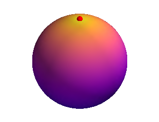
Sphere
(homogeneous space)
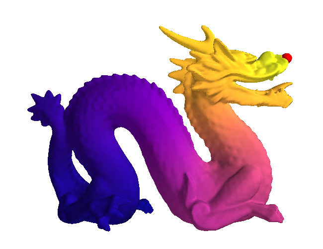
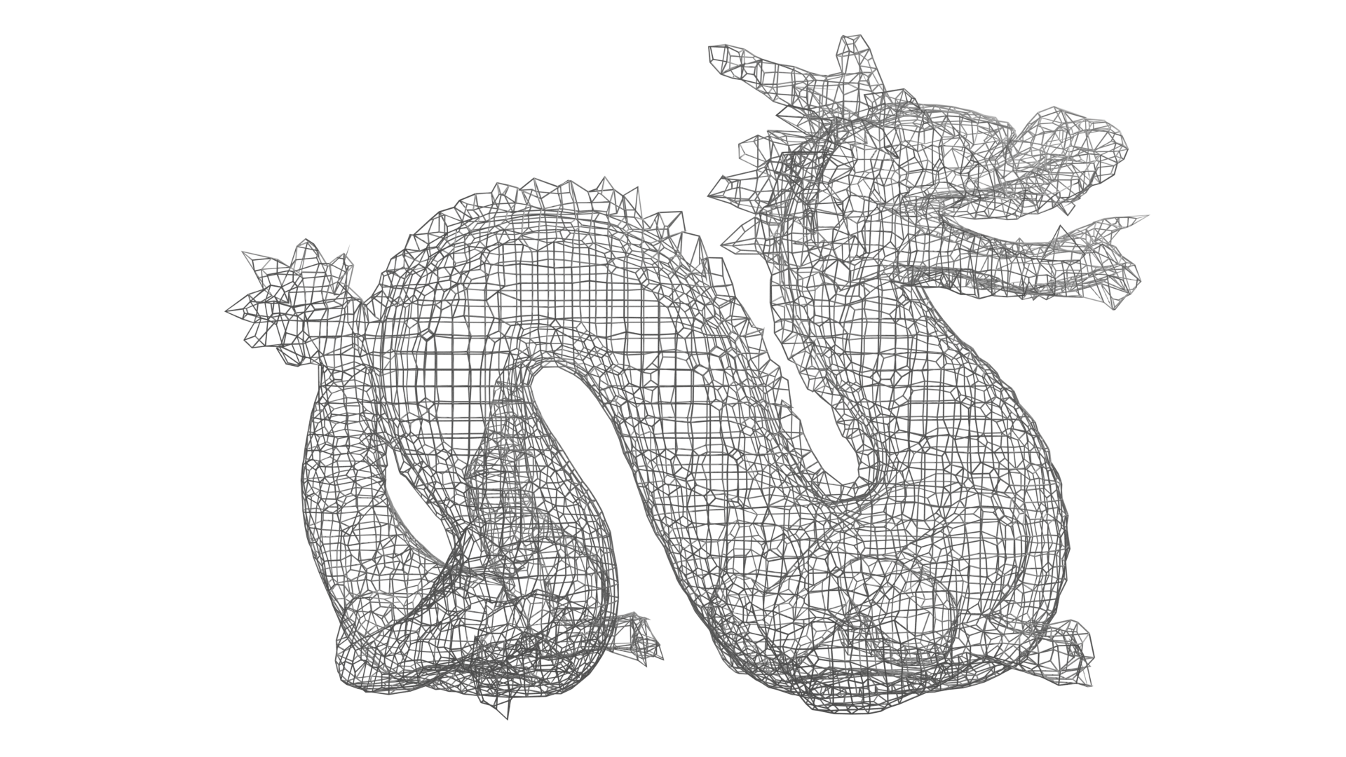
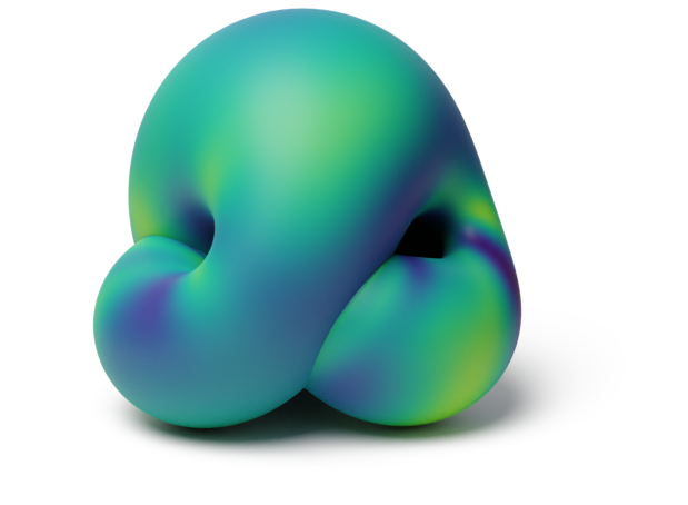
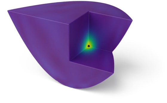
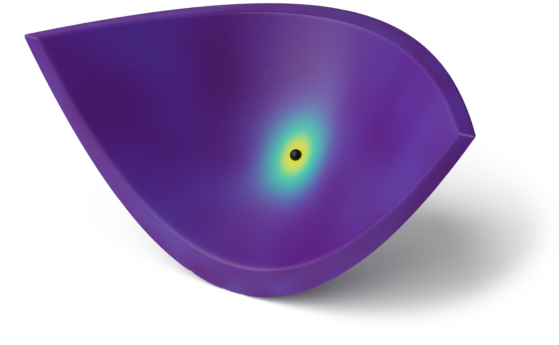
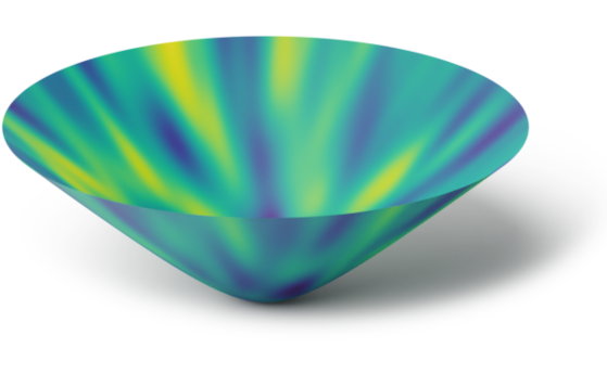
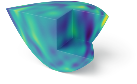
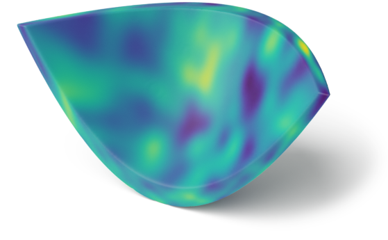
Dragon
(general manifold)
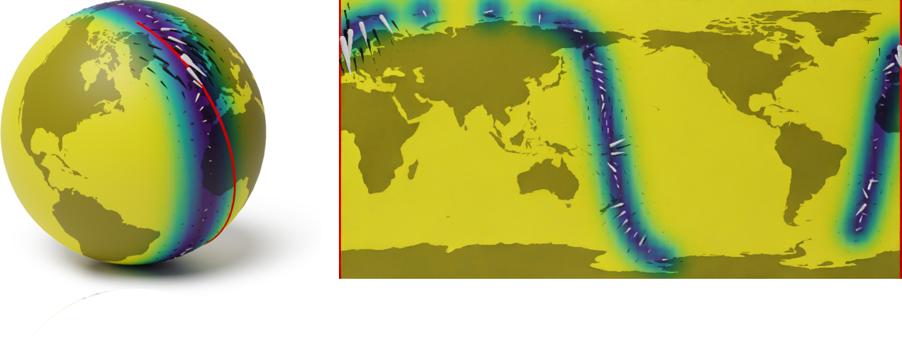
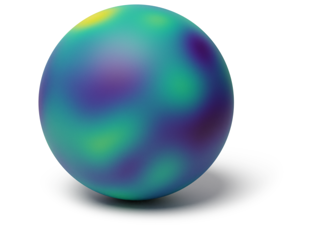 Sphere $\mathbb{S}_2$
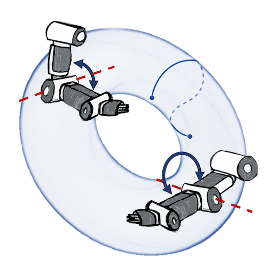
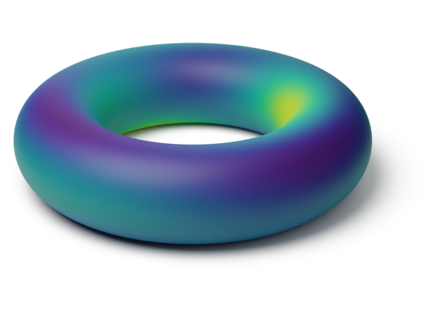 Torus $\mathbb{T}^2 = \bb{S}_1 \x \bb{S}_1$
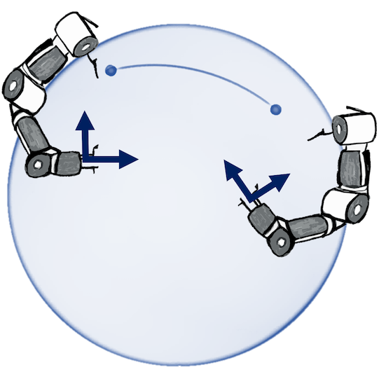
 Projective plane $\mathrm{RP}^2$
Examples: $\bb{H}_d$, $\mathrm{SPD}(d)$
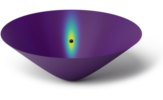 Hyperbolic space $\bb{H}_2$
Space of positive definite matrices $\f{SPD}(2)$
 Hyperbolic space $\bb{H}_2$
Space of positive definite matrices $\f{SPD}(2)$

Geometry-aware vs Euclidean
SPDE turns into a stochastic linear system. The solution has kernel $$ \htmlData{fragment-index=2,class=fragment}{ k_{\nu, \kappa, \sigma^2}(i, j) = \frac{\sigma^2}{C_{\nu, \kappa}} \sum_{n=0}^{\abs{V}-1} \Phi_{\nu, \kappa}(\lambda_n) \mathbf{f_n}(i)\mathbf{f_n}(j) } $$


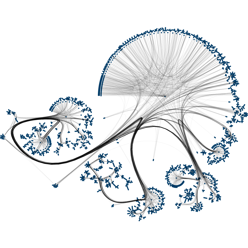
Consider the set of all unweighted graphs with $n$ nodes.
It is finite!
How to give it a geometric structure?
Make it into a space?

Beyond functions of actual graphs $f\big(\smash{\includegraphics[height=2.5em,width=1.0em]{figures/gg2.svg}}\big)$, it is useful to consider functions of equivalence classes of graphs: $f\big(\big\{\smash{\includegraphics[height=2.5em,width=1.0em]{figures/gg2.svg}}, \smash{\includegraphics[height=2.5em,width=1.0em]{figures/gg3.svg}}, \smash{\includegraphics[height=2.5em,width=1.0em]{figures/gg4.svg}}\big\}\big)$.


$$ \begin{aligned} \htmlData{fragment-index=1,class=fragment}{k(x,y)} &\htmlData{fragment-index=2,class=fragment}{ = \frac{\sigma^2}{C_{\nu, \kappa}} \sum_{n=0}^\infty \Phi_{\nu, \kappa}(\lambda_n) f_n(x) \mathrlap{f_n(y)} \htmlData{fragment-index=3,class=fragment}{ \obr{\phantom{f_n(y)}}{\hspace{-0.5cm}\text{spherical harmonics}\hspace{-0.5cm}} } } \\ &\htmlData{fragment-index=4,class=fragment}{= \frac{\sigma^2}{C_{\nu, \kappa}} \sum_{n=0}^\infty \Phi_{\nu, \kappa}(\lambda_n) \mathrlap{\del{\sum_{k=1}^{d_n} f_{n, k}(x) f_{n, k}(y)}} \htmlData{fragment-index=5,class=fragment}{ \ubr{\phantom{\del{\sum_{k=1}^{d_n} f_{n, k}(x) f_{n, k}(y)}}}{\hspace{-0.7cm} C_{n, d} \cdot \phi_{n, d}(x, y) \text{ --- zonal spherical harmonics}\hspace{-0.7cm}} } } \end{aligned} $$
The last equation
Circle
(Lie group)
Sphere
(homogeneous space)
Dragon
(general manifold)
Zonal spherical harmonics satisfy reproducing property:
$$ \begin{aligned} \htmlData{class=fragment}{ \phi_{n, d}(x, y) } & \htmlData{class=fragment}{ = C_{n, d} \int_{\mathbb{S^n}} \phi_{n, d}(x, u) \phi_{n, d}(y, u) d u } \\ & \htmlData{class=fragment}{ \approx \frac{C_{n, d}}{L} \sum_{l=1}^L \phi_{n, d}(x, u_l) \phi_{n, d}(y, u_l), } && \htmlData{class=fragment}{ u_l \stackrel{\text{i.i.d.}}{\sim} \mathrm{U}(\mathbb{S}_n). } \end{aligned} $$Hence $\sqrt{C_{n, d}/L} \cdot \phi_{n, d}(x, \v{u})$ forms an approximate feature transform.
This enables efficient sampling without knowing $f_n$. And this generalizes!
Sphere $\mathbb{S}_2$
Torus $\mathbb{T}^2 = \bb{S}_1 \x \bb{S}_1$
Projective plane $\mathrm{RP}^2$