HEC-DSA, Université de Lausanne
Gaussian Processes
in Machine Learning
Viacheslav Borovitskiy (Slava)


Definition. A Gaussian process is random function $f : X \times \Omega \to \R$ such that for any $x_1,..,x_n$, the vector $f(x_1),..,f(x_n)$ is multivariate Gaussian.
The distribution of a Gaussian process is characterized by
Notation: $f \~ \f{GP}(m, k)$.
The kernel $k$ must be positive (semi-)definite, i.e. for all $x_1, .., x_n \in X$
the matrix $K_{\v{x} \v{x}} := \cbr{k(x_i, x_j)}_{\substack{1 \leq i \leq n \\ 1 \leq j \leq n}}$ must be positive (semi-)definite.
Takes
giving the posterior (conditional) Gaussian process $\f{GP}(\hat{m}, \hat{k})$.
The functions $\hat{m}$ and $\hat{k}$ may be explicitly expressed in terms of $m$ and $k$.
Goal: minimize unknown function $\phi$ in as few evaluations as possible.


Also
$$
\htmlData{class=fragment fade-out,fragment-index=9}{
\footnotesize
\mathclap{
k_{\nu, \kappa, \sigma^2}(x,x') = \sigma^2 \frac{2^{1-\nu}}{\Gamma(\nu)} \del{\sqrt{2\nu} \frac{\norm{x-x'}}{\kappa}}^\nu K_\nu \del{\sqrt{2\nu} \frac{\norm{x-x'}}{\kappa}}
}
}
\htmlData{class=fragment d-print-none,fragment-index=9}{
\footnotesize
\mathclap{
k_{\infty, \kappa, \sigma^2}(x,x') = \sigma^2 \exp\del{-\frac{\norm{x-x'}^2}{2\kappa^2}}
}
}
$$
$\sigma^2$: variance
$\kappa$: length scale
$\nu$: smoothness
$\nu\to\infty$: Gaussian kernel (RBF)

$\nu = 1/2$

$\nu = 3/2$

$\nu = 5/2$

$\nu = \infty$
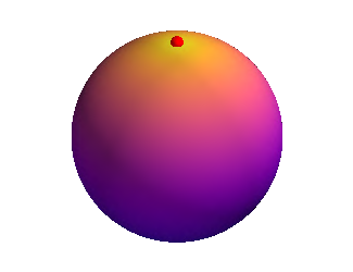
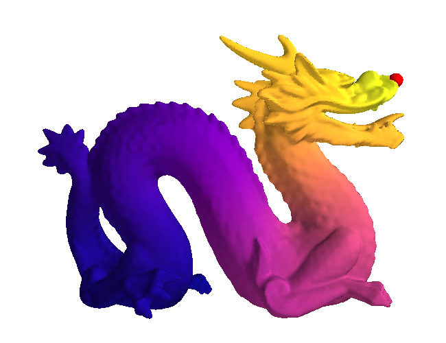
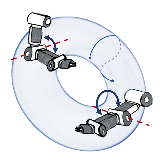
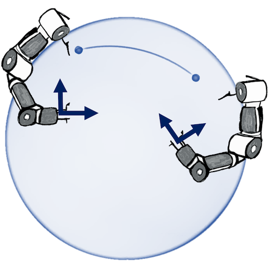
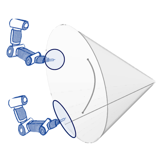
$$ k_{\infty, \kappa, \sigma^2}^{(d_g)}(x,x') = \sigma^2\exp\del{-\frac{d_g(x,x')^2}{2\kappa^2}} $$
Theorem. (Feragen et al.) Let $M$ be a complete Riemannian manifold without boundary. If $k_{\infty, \kappa, \sigma^2}^{(d_g)}$ is positive semi-definite for all $\kappa$, then $M$ is isometric to a Euclidean space.
$$ \htmlData{class=fragment,fragment-index=0}{ \underset{\t{Matérn}}{\undergroup{\del{\frac{2\nu}{\kappa^2} - \Delta}^{\frac{\nu}{2}+\frac{d}{4}} f = \c{W}}} } $$ $\Delta$: Laplacian $\c{W}$: Gaussian white noise
$$ \htmlData{class=fragment,fragment-index=0}{ \del{\frac{2\nu}{\kappa^2} - \Delta}^{\frac{\nu}{2}+\frac{d}{4}} f = \c{W} } $$
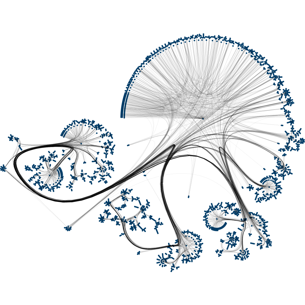
| Riemannian Manifolds | Undirected Graphs |
|---|---|
| • $\Delta$ — Laplace–Beltrami, | • $\Delta$ — graph Laplacian, |
| • $\c{W}$ — white noise controlled by the Riemannian volume, | • $\c{W}$ — i.i.d. Gaussians, |
|
• $\left( \frac{2 \nu}{\kappa^2} - \Delta \right)^{\frac{\nu}{2} + \frac{d}{4}}$ is defined via functional calculus |
|
Define $\underbrace{H^s(M)}_{\text{Sobolev space}} = \underbrace{(1-\Delta)^{-\frac{s}{2}}}_{\text{Bessel potential}} L^2(M)$
Then the solution of $$ \bigg(\frac{2\nu}{\kappa^2} - \Delta\bigg)^{\frac{\nu}{2}+\frac{d}{4}} f = \c{W} $$
At least the solution of $$ \bigg(1 - \Delta\bigg)^{\frac{\nu}{2}+\frac{d}{4}} f = \c{W} $$
May be regarded as the isonormal proces on $H^{\nu + d/2}$.
It has the reproducing kernel of $H^{\nu + d/2}$ as its kernel.
The solution is a Gaussian process with kernel $$ \htmlData{class=fragment}{ k_{\nu, \kappa, \sigma^2}(x,x') = \frac{\sigma^2}{C_\nu} \sum_{n=0}^\infty \del{\frac{2\nu}{\kappa^2} - \lambda_n}^{-\nu-\frac{d}{2}} f_n(x) f_n(x') } $$
The solution is a Gaussian process with kernel $$ \htmlData{class=fragment}{ k_{\nu, \kappa, \sigma^2}(x,x') = \frac{\sigma^2}{C_\nu} \sum_{n=0}^\infty \del{\frac{2\nu}{\kappa^2} - \lambda_n}^{-\nu-\frac{d}{2}} f_n(x) f_n(x') } $$
Proof. 1. Show that the covariance function of the solution is the reproducing kernel of the Sobolev space $H^{\nu + d/2}$.
2. The reproducing kernel may be computed via the Fourier method (known).

The solution is a Gaussian process with kernel $$ \htmlData{class=fragment}{ k_{\nu, \kappa, \sigma^2}(i, j) = \frac{\sigma^2}{C_{\nu}} \sum_{n=0}^{\abs{V}-1} \del{\frac{2\nu}{\kappa^2} + \mathbf{\lambda_n}}^{-\nu} \mathbf{f_n}(i)\mathbf{f_n}(j) } $$


$$ \htmlData{fragment-index=0,class=fragment}{ x_0 } \qquad \htmlData{fragment-index=1,class=fragment}{ x_1 = x_0 + f(x_0)\Delta t } \qquad \htmlData{fragment-index=2,class=fragment}{ x_2 = x_1 + f(x_1)\Delta t } \qquad \htmlData{fragment-index=3,class=fragment}{ .. } $$


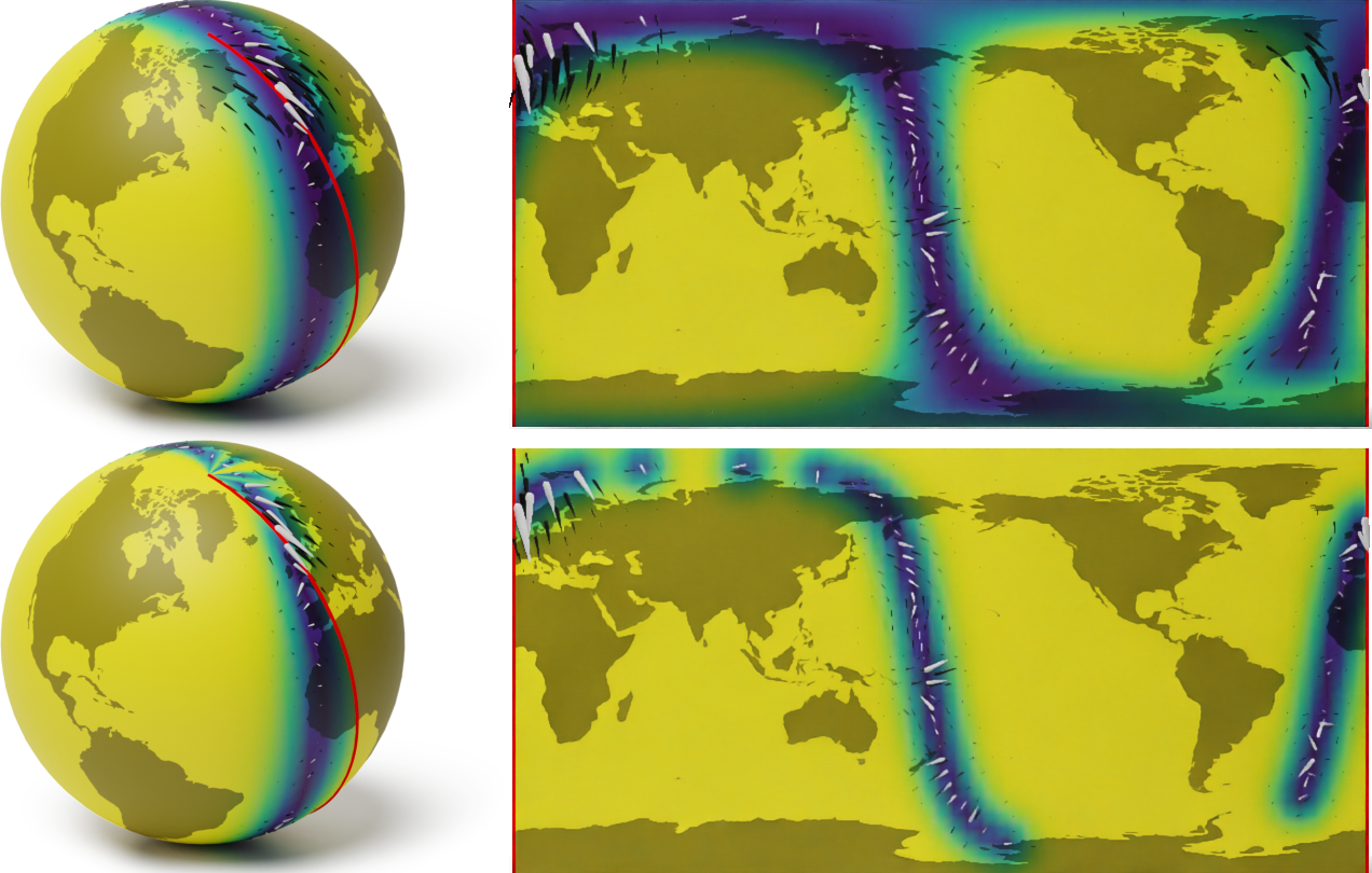
A naive Euclidean model
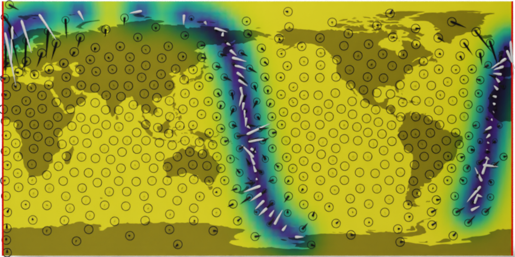
Wind speed extrapolation on a map
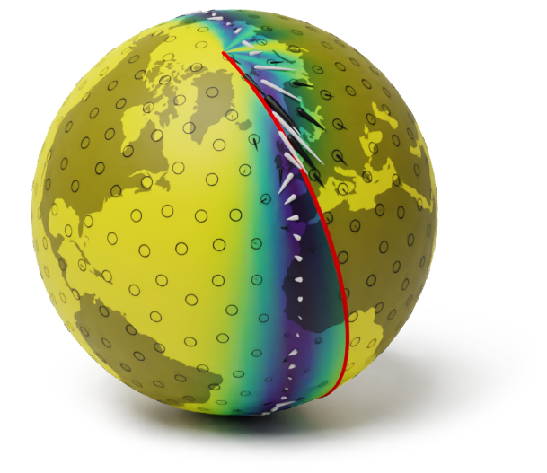
The corresponding model on a globe
A geometry-aware model
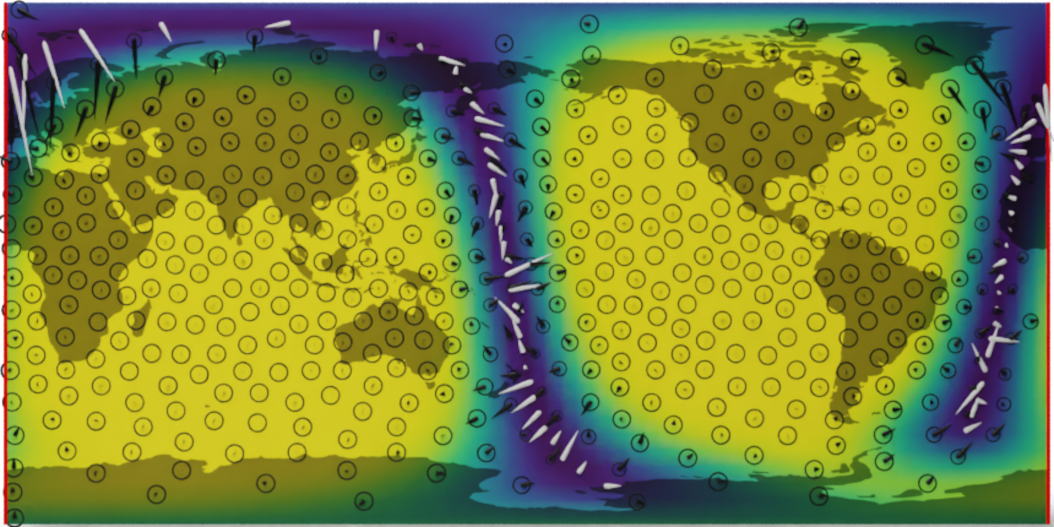
Wind speed extrapolation on a map
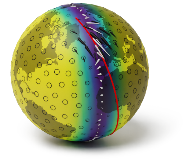
The corresponding model on a globe
Interpolation: $f \given f(\v{x}) = \v{y}$


$\hat{m} = \argmin\limits_{f \in \c{H}_k} \norm{f}_{\c{H}_k}$ subject to $f(x_i) = y_i$
$(\hat{m}(x) - f_{\text{true}}(x))^2 \leq \norm{f_{\text{true}}}_{\c{H}_k}^2 \hat{k}(x, x)$
Regression: $f \given f(\v{x}) + \v{\varepsilon} = \v{y}~~$ where $~~\v{\varepsilon} \sim \f{N}(0, \sigma_n^2 I)$


$\hat{m} = \argmin\limits_{f \in \c{H}_k} \sum\limits_{i=1}^n (f(x_i) - y_i)^2 + \sigma_n^2 \norm{f}_{\c{H}_k}$
$(\hat{m}(x) - f_{\text{true}}(x))^2 \leq \norm{f_{\text{true}}}_{\c{H}_{k^{\sigma}}}^2 \! \del{\hat{k}(x, x) \!+\! \sigma_n^2}$
Here $\c{H}_{k^{\sigma}} = \c{H}_{k} + \c{H}_{\sigma_n^2 \delta}$
and $x \not= x_i, i = 1, \ldots, n$
Moments $\hat{m}(x)$ and $\hat{k}(x, x)$ of the posterior Gaussian process
may be expressed in terms of the RKHS $\c{H}_k$.
Consider a covariance $k$ living on a compact space $\c{X}$ with a finite measure $\nu$.
A generalized Driscol’s Zero-One Law. Consider $f \sim \f{GP}(0, k)$ and $r$ such that $\c{H}_k \subseteq \c{H}_r$. Let $I_{k r}: \c{H}_k \to \c{H}_r$ be the natural inclusion operator.
Thus $f \in \c{H}_k$ with probability $0$, however...
For any $0 < \theta < 1$ we have with probability $1$: $f \in (\c{H}_k, L^2(\c{X}, \nu))_{\theta, 2}$.


Own works:
V. Borovitskiy, A. Terenin, P. Mostowsky, M. P. Deisenroth. Matérn Gaussian Processes on Riemannian Manifolds.
In Neural Information Processing Systems (NeurIPS) 2020.
V. Borovitskiy, I. Azangulov, A. Terenin, P. Mostowsky, M. P. Deisenroth. Matérn Gaussian Processes on Graphs.
In International Conference on Artificial Intelligence and Statistics (AISTATS) 2021.
M. Hutchinson, A. Terenin, V. Borovitskiy, S. Takao, Y. W. Teh, M. P. Deisenroth. Vector-valued Gaussian Processes on Riemannian Manifolds via Gauge-Independent Projected Kernels. To appear in NeurIPS 2021.
Other works:
M. Kanagawa, P. Hennig, D. Sejdinovic, B. K. Sriperumbudur. Gaussian Processes and Kernel Methods: A Review on Connections and Equivalences. arXiv preprint arXiv:1807.02582, 2018.
I. Steinwart. Convergence Types and Rates in Generic Karhunen-Loeve Expansions with Applications to Sample Path Properties. Potential Analysis, 2018.
F. Lindgren, H. Rue, J. Lindström. An explicit link between Gaussian fields and Gaussian Markov random fields: the stochastic partial differential equation approach. Journal of the Royal Statistical Society: Series B, 2011.
A. Feragen, F. Lauze, S. Hauberg. Geodesic exponential kernels: When curvature and linearity conflict. Proceedings of the IEEE conference on computer vision and pattern recognition, 2015.
P. Whittle. On Stationary Processes in the Plane. Biometrika, 1954.
viacheslav.borovitskiy@gmail.com https://vab.im