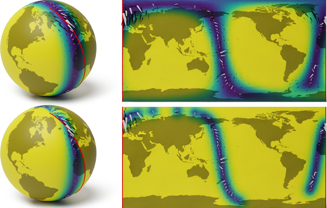
Problem: model geology deep underground.
Data: measurements from sparse wells.

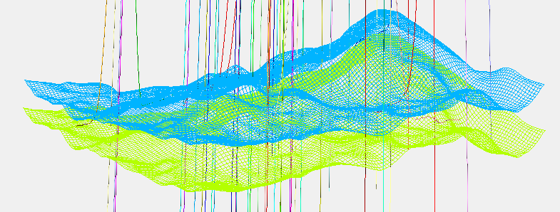
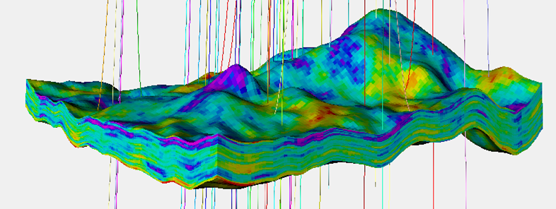
One deterministic answer is not an option!

Definition. A Gaussian process is random function $f : X \times \Omega \to \R$ such that for any $x_1,..,x_n$, the vector $f(x_1),..,f(x_n)$ is multivariate Gaussian.

The distribution of a Gaussian process is characterized by

• a mean function $m(x) = \E(f(x))$,
• a kernel (covariance) function $k(x, x') = \Cov(f(x), f(x'))$,

Notation: $f \~ \f{GP}(m, k)$.

Takes

• a prior Gaussian Process $\f{GP}(m, k)$
• and data $(x_1, y_1), .., (x_n, y_n) \in X \x \R$,

giving the posterior Gaussian process $\f{GP}(\tilde{m}, \tilde{k})$.

The functions $\tilde{m}$ and $\tilde{k}$ may be explicitly expressed in terms of $m$ and $k$.

Goal: minimize unknown function $\phi$ in as few evaluations as possible.

1. Build GP posterior $f \given \v{y}$ using data $(x_1,\phi(x_1)),..,(x_n,\phi(x_n))$.
2. Choose $$\htmlClass{fragment}{ x_{n+1} = \argmax_{x\in\c{X}} \underbrace{\alpha_{f\given\v{y}}(x).}_{\text{acquisition function}} }$$ For instance, expected improvement $$\alpha_{f\given\v{y}}(x) = \E_{f\given\v{y}} \max(0, {\displaystyle\min_{i=1,..,n}} \phi(x_i) - f(x)).$$

Assume we have data $(x_1, y_1), .., (x_n, y_n)$ and the standard Bayesian model $$y_i = f(x_i) + \varepsilon_i, \qquad f \sim \f{GP}(0, k), \qquad \varepsilon_i \stackrel{\text{i.i.d.}}{\sim} \f{N}(0, \sigma^2).$$

The posterior Gaussian process $f \sim \f{GP}(\tilde{m}, \tilde{k})$ is then used for predictions $$\begin{aligned} \tilde{m}(a)~=~&k(a, \v{x}) \del{k(\v{x}, \v{x}) + \sigma^2 I}^{-1} \v{y}, \\ \tilde{k}(a, b) ~=~ k(a, b) - &\underbrace{k(a, \v{x})}_{\text{vector}~1 \x n} (\underbrace{k(\v{x}, \v{x}) + \sigma^2 I}_{\text{matrix}~n \x n})^{-1} \underbrace{k(\v{x}, b)}_{\text{vector}~n \x 1}. \end{aligned}$$

Notation: $\v{x} \stackrel{\text{def}}{=} (x_1, .., x_n)^{\top}$ and $k(\v{x}, \v{x}) \stackrel{\text{def}}{=} \del{k(x_i, x_j)}_{\substack{1 \leq i \leq n \\ 1 \leq j \leq n}}$.

Idea. Approximate the posterior process $\f{GP}(\tilde{m}, \tilde{k})$ with a simpler process belonging to some parametric family $\f{GP}(m_{\theta}, k_{\theta})$.

Take a vector $\v{z} = (z_1, .., z_m)^{\top}$ of pseudo-locations, $m \ll n$.
Consider pseudo-observations $\v{u} = (u_1, .., u_m)^{\top} \sim \f{N}(\v{\mu}, \m{\Sigma})$.

Put $\theta = (\v{z}, \v{\mu}, \m{\Sigma})$ and $f_{\theta}$ to be the posterior under Bayesian model $$\begin{aligned} u_i = f(z_i), && f \sim \f{GP}(0, k), && \v{u} = (u_1, .., u_m)^{\top} \sim \f{N}(\v{\mu}, \m{\Sigma}) \end{aligned}$$

We have $\tilde{f}_{\theta} \sim \f{GP}(m_{\theta}, k_{\theta})$ with $$\begin{alignedat}{3} m_{\theta}(a) &= k(a, \v{z}) &&k(\v{z}, \v{z})^{-1} \v{\mu}, \\ k_{\theta}(a, b) &= k(a, b) &&- k(a, \v{z}) k(\v{z}, \v{z})^{-1} k(\v{z}, b) \\ &&&+ k(a, \v{z}) \underbrace{ k(\v{z}, \v{z})^{-1} \m{\Sigma} k(\v{z}, \v{z})^{-1} }_{\text{matrix}~m \x m} k(\v{z}, b). \end{alignedat}$$ If $\v{z}, \v{\mu}, \m{\Sigma}$ are given, computing approximate posterior is $O(m^3)$.

The optimization problem is $D_{KL}(f_{\theta}||\tilde{f}) \to \min$. $$\begin{aligned} D_{KL}(f_{\theta}||\tilde{f}) \stackrel{\text{thm}}{=}& D_{KL}(f_{\theta}(\v{x} \oplus \v{z})||\tilde{f}(\v{x} \oplus \v{z})) \\ \stackrel{\text{thm}}{=}& D_{KL}(N(\v{\mu}, \m{\Sigma})||N(0, k(\v{z}, \v{z}))) \\ & - \sum_{i=1}^n \E \ln p_{\f{N}(f(x_i), \sigma^2)}(y_i) + C. \end{aligned}$$

Can be solved by stochastic gradient descent with iteration cost $O(m^3)$.

Result. We approximate the posterior process $\f{GP}(\tilde{m}, \tilde{k})$ with a simpler process belonging to a certain parametric family $\f{GP}(m_{\theta}, k_{\theta})$.

Take $f \sim \f{GP}(m, k)$ and a finite set of locations $\v{v} = (v_1, .., v_s)$.

Restricting $f$ to $\v{v}$ we get the random vector $f(\v{v}) \sim \f{N}(m(\v{v}), k(\v{v}, \v{v}))$.

Then $$\begin{aligned} f(\v{v}) \stackrel{\text{d}}{=} m(\v{v}) + k(\v{v}, \v{v})^{1/2} \v{\varepsilon}, && \v{\varepsilon} \sim \f{N}(\v{0}, \m{I}) \end{aligned}.$$

Problem: it takes $O(s^3)$ to find $k(\v{v}, \v{v})^{1/2}$ and the sample lives on a grid.

Priors are usually assumed stationary. If $f \sim \f{GP}(0, k)$ is stationary, then $$\begin{aligned} k(a, b) = \int e^{2 \pi i \langle a-b, \xi \rangle} s(\xi) \mathrm{d} \xi \approx \frac{1}{l} \sum_{j=1}^l e^{2 \pi i \langle a-b, \xi_j \rangle}, && \xi_j \stackrel{\text{i.i.d.}}{\sim} s(\xi). \end{aligned}$$

This gives the approximation for the random process itself $$\begin{aligned} f(a) = \frac{1}{l} \sum_{j=1}^l w_j e^{2 \pi i \langle a, \xi_j \rangle}, && w_j \stackrel{\text{i.i.d.}}{\sim} \f{N}(0,1), && \xi_j \stackrel{\text{i.i.d.}}{\sim} s(\xi). \end{aligned}$$

It takes only $O(s l)$ to sample on grid of size $s$. And we do not need a grid!

The posterior Gaussian process $\tilde{f} \sim \f{GP}(\tilde{m}, \tilde{k})$ can be expressed by $$\tilde{f}(a) \stackrel{\text{d}}{=} f(a) + k(a, \v{x}) \del{k(\v{x}, \v{x}) + \sigma^2 I}^{-1} (\v{y} - f(\v{x}) -\v{\varepsilon}),$$ where $\v{\varepsilon} \stackrel{\text{i.i.d.}}{\sim} \f{N}(0, \sigma^2)$.

With this, o sample on grid of size $s$ with $n$ data points $O(s l + n^3)$.

Can we improve $O(n^3)$ scaling in this case?

Proposition. A sample from the $f_{\theta}$ may be obtained as follows.

1. Sample $\v{u} = (u_1, .., u_m) \sim \f{N}(\v{\mu}, \m{\Sigma})$,
2. Return a sample from the posterior Gaussian process with $(z_1, u_1), .., (z_m, u_m)$ as data.

Manifolds

Graphs

How should we build and use Gaussian process models in these settings?