Motivating Example
Consider a Simple Dynamical System: a Pendulum
$$ \htmlData{fragment-index=0,class=fragment}{ x_0 } \qquad \htmlData{fragment-index=1,class=fragment}{ x_1 = x_0 + f(x_0)\Delta t } \qquad \htmlData{fragment-index=2,class=fragment}{ x_2 = x_1 + f(x_1)\Delta t } \qquad \htmlData{fragment-index=3,class=fragment}{ .. } $$
Consider a Simple Dynamical System: a Pendulum
$$ x_0 \qquad x_1 = x_0 + f(x_0)\Delta t \qquad x_2 = x_1 + f(x_1)\Delta t \qquad .. $$
Consider a Simple Dynamical System: a Pendulum
assume $f$ unknown, model $f$ as a GP.
$$ x_0 \qquad x_1 = x_0 + f(x_0)\Delta t \qquad x_2 = x_1 + f(x_1)\Delta t \qquad .. $$
Pendulum Dynamics: Phase Portrait
Pendulum Dynamics: Phase Portrait
Pendulum Dynamics: Phase Portrait
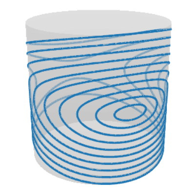
Pendulum Dynamics: Phase Portrait
Phase portrait is periodic!

I.e. the state space is actually a cylinder!
Need priors on non-Euclidean domains!
Be able to: evaluate $k(x, x')$, differentiate it, sample $\mathrm{GP}(0, k)$.
Non-Euclidean Domains

Manifolds
e.g. in physics (robotics)
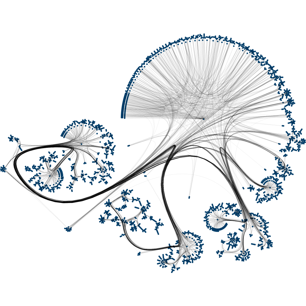
Graphs
e.g. for road networks.
Spaces of graphs
e.g. for drug design
Standard Priors
Matérn Gaussian Processes
$$
\htmlData{class=fragment fade-out,fragment-index=6}{
\footnotesize
\mathclap{
k_{\nu, \kappa, \sigma^2}(x,x') = \sigma^2 \frac{2^{1-\nu}}{\Gamma(\nu)} \del{\sqrt{2\nu} \frac{\abs{x-x'}}{\kappa}}^\nu K_\nu \del{\sqrt{2\nu} \frac{\abs{x-x'}}{\kappa}}
}
}
\htmlData{class=fragment d-print-none,fragment-index=6}{
\footnotesize
\mathclap{
k_{\infty, \kappa, \sigma^2}(x,x') = \sigma^2 \exp\del{-\frac{\abs{x-x'}^2}{2\kappa^2}}
}
}
$$
$\sigma^2$: variance
$\kappa$: length scale
$\nu$: smoothness
$\nu\to\infty$: RBF kernel (Gaussian, Heat, Diffusion)
$\nu = 1/2$
$\nu = 3/2$
$\nu = 5/2$
$\nu = \infty$
How to generalize these
to non-Euclidean settings?
Distance-based Approach
$$ k_{\infty, \kappa, \sigma^2}(x,x') = \sigma^2\exp\del{-\frac{|x - x'|^2}{2\kappa^2}} $$
$$ k_{\infty, \kappa, \sigma^2}^{(d)}(x,x') = \sigma^2\exp\del{-\frac{d(x,x')^2}{2\kappa^2}} $$
For manifolds. Not well-defined unless the manifold is isometric to a Euclidean space.
(Feragen et al. 2015)
For graphs. Not well-defined unless nodes can be isometrically embedded into a Hilbert space.
(Schonberg, 1930s)
For spaces of graphs. What is a space of graphs?!
Need a different generalization
Another Approach: Stochastic Partial Differential Equations
$$ \htmlData{class=fragment,fragment-index=0}{ \underset{\t{Matérn}}{\undergroup{\del{\frac{2\nu}{\kappa^2} - \Delta}^{\frac{\nu}{2}+\frac{d}{4}} f = \c{W}}} } $$ $\Delta$: Laplacian $\c{W}$: Gaussian white noise $d$: dimension
Generalizes well
Geometry-aware: respects to symmetries of the space
Implicit: no formula for the kernel
Making It Explicit:
Compact Manifolds
Examples: $\bb{S}_d$, $\bb{T}^d$
Solution for Compact Riemannian Manifolds
The solution is a Gaussian process with kernel $$ \htmlData{fragment-index=2,class=fragment}{ k_{\nu, \kappa, \sigma^2}(x,x') = \frac{\sigma^2}{C_{\nu, \kappa}} \sum_{n=0}^\infty \Phi_{\nu, \kappa}(\lambda_n) f_n(x) f_n(x') } $$
$\lambda_n, f_n$: eigenvalues and eigenfunctions of the Laplace–Beltrami operator
$$ \htmlData{fragment-index=4,class=fragment}{ \Phi_{\nu, \kappa}(\lambda) = \begin{cases} \htmlData{fragment-index=5,class=fragment}{ \del{\frac{2\nu}{\kappa^2} - \lambda}^{-\nu-\frac{d}{2}} } & \htmlData{fragment-index=5,class=fragment}{ \nu < \infty \text{ --- Matérn} } \\ \htmlData{fragment-index=6,class=fragment}{ e^{-\frac{\kappa^2}{2} \lambda} } & \htmlData{fragment-index=6,class=fragment}{ \nu = \infty \text{ --- Heat (RBF)} } \end{cases} } $$How to get $\lambda_n, f_n$?
Answer I: Discretize the Problem
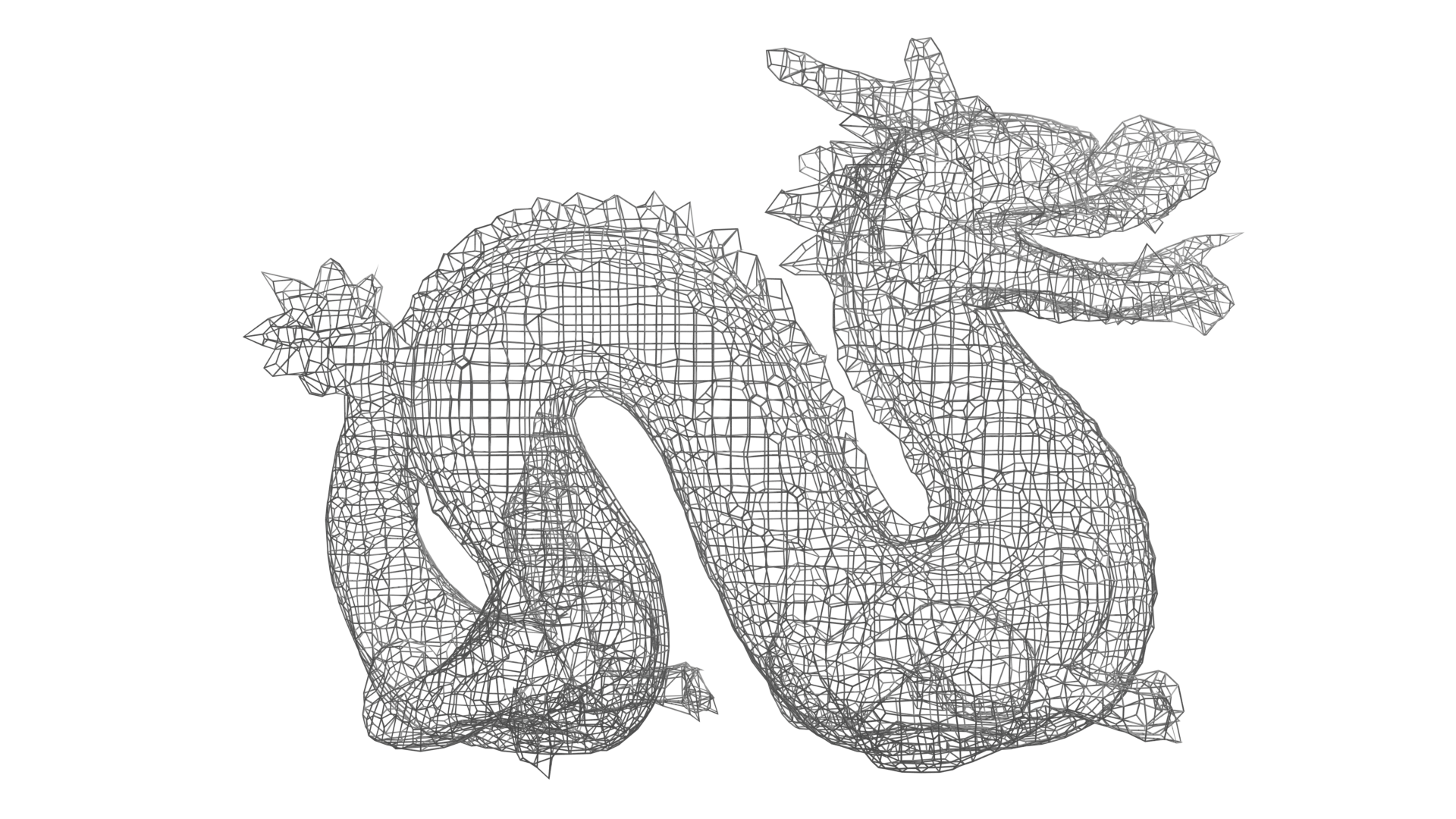
Mesh the manifold, consider the discretized Laplace–Beltrami (a matrix).
Answer II: Use Algebraic Structure
For manifolds with rich group of symmetries, termed homogeneous spaces.
These include
- Lie groups, like rotations $\mathrm{SO}(n)$ and unitary matrices $\mathrm{SU}(n)$,
- "Proper" homogeneous spaces, e.g. spheres $\mathbb{S}_d$, projective spaces $\mathrm{RP}_d$, Stiefel manifolds $\mathrm{V}(k, n)$ or Grassmannians $\mathrm{Gr}(n, r)$.
$\lambda_n, f_n$ are connected to representation theory of the group of symmetries.
Examples: The Values of $k_{1/2}(\htmlStyle{color:rgb(255, 19, 0)!important}{\bullet},\.)$ on Compact Riemannian Manifolds
Circle
(Lie group)
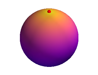
Sphere
(homogeneous space)
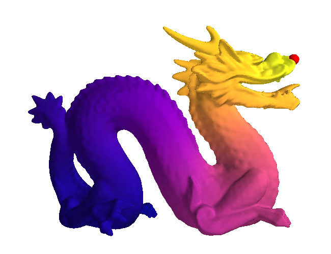
Dragon
(general manifold)
Examples: Samples from $\mathrm{GP}(0, k_{\infty})$ on Compact Homgeneous Spaces
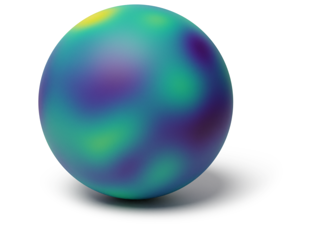 Sphere $\mathbb{S}_2$
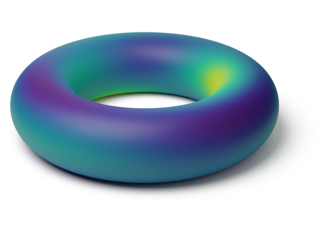 Torus $\mathbb{T}^2 = \bb{S}_1 \x \bb{S}_1$
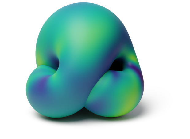 Projective plane $\mathrm{RP}^2$
Driven by generalized random phase Fourier features (GRPFF).
Making It Explicit:
Non-compact Manifolds
Examples: $\bb{H}_d$, $\mathrm{SPD}(d)$
Random Fourier Features (RFF)
Take stationary $k$. Assume for simplicity $k(x, x) = 1$. Then
$$ \htmlData{data-id=rffformula,class=fragment}{ \begin{aligned} k(x, x') &= \int_{\R^d} S(\lambda) e^{2 \pi i \innerprod{x - x'}{\lambda}} \d \lambda \\ & \htmlData{class=fragment}{ \approx \frac{1}{L} \sum_{l=1}^L e^{2 \pi i \innerprod{x - x'}{\lambda_l}} \qquad \lambda_l \sim S(\lambda) } \end{aligned} } $$$k$ is RBF $\implies$ $S(\lambda)$ is Gaussian. $k$ is Matérn $\implies$ $S(\lambda)$ is $t$ distributed.
Random Fourier Features (RFF) for Symmetric Spaces
$k$ is RBF $\implies$ $S(\lambda)$ is Gaussian. $k$ is Matérn $\implies$ $S(\lambda)$ is $t$ distributed.
• $\pi^{(\lambda)}$ is an explicit integral.
• $c(\lambda)$ has closed form.
• $c(\lambda)^{-2} S(\lambda)$ is a non-standard, potentially unnormalized, density.
Examples: The Values of $k_{\infty}(\htmlStyle{color:rgb(0, 0, 0)!important}{\bullet},\.)$ on Non-compact Manifolds
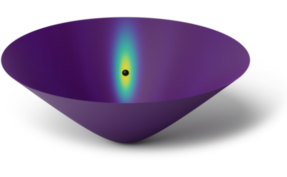 Hyperbolic space $\bb{H}_2$

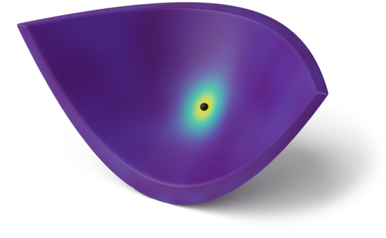
Space of positive definite matrices $\f{SPD}(2)$
Random Fourier Features for Sampling
Since $e^{2 \pi i \innerprod{x - x'}{\lambda_l}} = e^{2 \pi i \innerprod{x}{\lambda_l}} \overline{e^{2 \pi i \innerprod{x'}{\lambda_l}}}$, the above is an inner product.
$$ \htmlData{class=fragment}{ f(x) \approx \frac{1}{\sqrt{L}} \sum_{l=1}^L w_l e^{2 \pi i \innerprod{x}{\lambda_l}} \qquad w_l \sim \mathrm{N}(0, 1) \qquad \lambda_l \sim S(\lambda) } $$
Random Fourier Features for Sampling: symmetric spaces
Since $ \htmlData{fragment-index=3,class=fragment fade-out disappearing-fragment}{ e^{2 \pi i \innerprod{x - x'}{\lambda_l}} } \htmlData{fragment-index=3,class=fragment fade-in appearing-fragment}{ {\color{blue}\pi^{(\lambda_l)}(x, x')} } \!\,= \htmlData{fragment-index=4,class=fragment fade-out disappearing-fragment}{ e^{2 \pi i \innerprod{x}{\lambda_l}} \overline{e^{2 \pi i \innerprod{x'}{\lambda_l}}} } \htmlData{fragment-index=4,class=fragment fade-in appearing-fragment}{ {\color{blue} \pi^{(\lambda_l)}(x, ?) \overline{\pi^{(\lambda_l)}(x', ?)} } } $, the above is an inner product. $ \vphantom{ e^{2 \pi i \innerprod{x - x'}{\lambda_l}} {\color{blue}\pi^{(\lambda_l)}(x, x')} \!\,= e^{2 \pi i \innerprod{x}{\lambda_l}} \overline{e^{2 \pi i \innerprod{x'}{\lambda_l}}} {\color{blue} \pi^{(\lambda_l)}(x, ?) \overline{\pi^{(\lambda_l)}(x', ?)} } } \sout{ {\color{blue}\pi^{(\lambda_l)}(x, x')} = {\color{blue} \pi^{(\lambda_l)}(x, ?) \overline{\pi^{(\lambda_l)}(x', ?)} } } $, $ \vphantom{ e^{2 \pi i \innerprod{x - x'}{\lambda_l}} {\color{blue}\pi^{(\lambda_l)}(x, x')} \!\,= e^{2 \pi i \innerprod{x}{\lambda_l}} \overline{e^{2 \pi i \innerprod{x'}{\lambda_l}}} {\color{blue} \pi^{(\lambda_l)}(x, ?) \overline{\pi^{(\lambda_l)}(x', ?)} } } {\color{blue}\pi^{(\lambda_l)}(x, x')} = \E_{h \sim \mu_H} e^{\innerprod{i \lambda + \rho}{\,a(h, x)}} \overline{ e^{\innerprod{i \lambda + \rho}{\,a(h, x')}} }, $ where
$$ f(x) \approx \frac{1}{\sqrt{L}} \sum_{l=1}^L w_l e^{2 \pi i \innerprod{x}{\lambda_l}} \qquad w_l \sim \mathrm{N}(0, 1) \qquad \lambda_l \sim S(\lambda) $$
• the vector $\rho$ and the function $a(\cdot, \cdot)$ are known,
• $\mu_H$ is samplabale.
• Monte Carlo approximation of the expectation $\E_{h \sim \mu_H}$ is an inner product.
Examples: Samples from $\mathrm{GP}(0, k_{\infty})$ on Non-compact Homgeneous Spaces
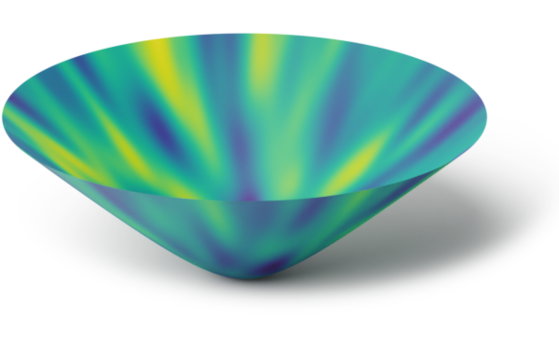 Hyperbolic space $\bb{H}_2$
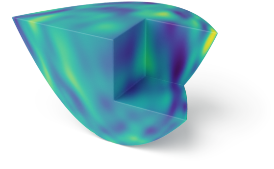
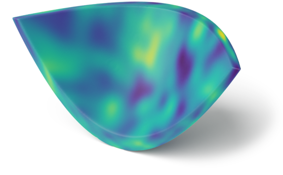
Space of positive definite matrices $\f{SPD}(2)$
Applications: Bayesian Optimization in Robotics
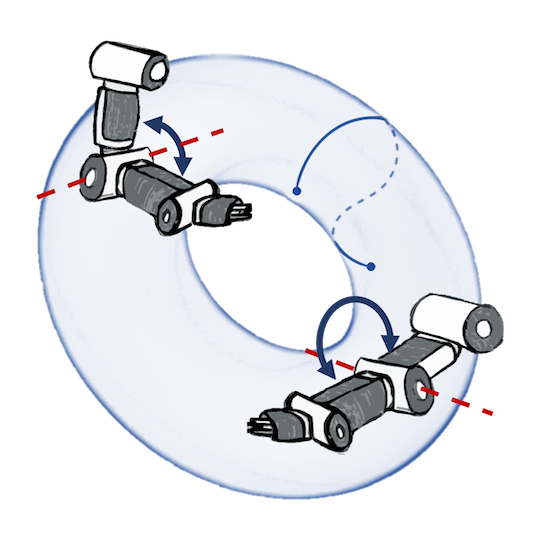
Joint postures: $\mathbb{T}^d$
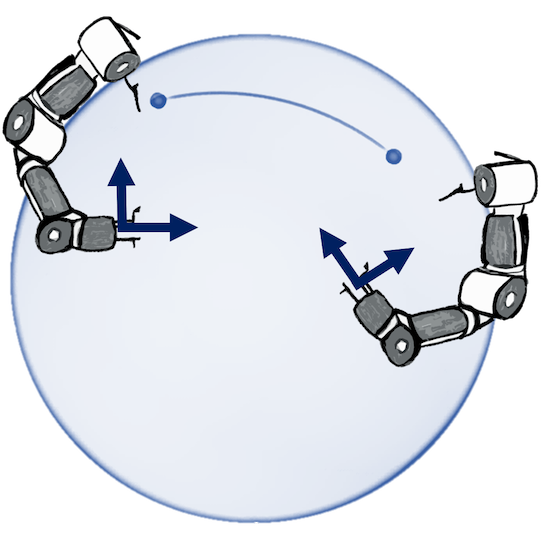
Rotations: $\mathbb{S}_3$, $\operatorname{SO}(3)$

Manipulability: $\operatorname{SPD(3)}$
Application: Wind Speed Modeling (Vector Fields on Manifolds)

Geometry-aware vs Euclidean
Making It Explicit:
Node Sets of Graphs
Matérn Kernels on Weighted Undirected Graphs
SPDE turns into a stochastic linear system. The solution has kernel $$ \htmlData{fragment-index=2,class=fragment}{ k_{\nu, \kappa, \sigma^2}(i, j) = \frac{\sigma^2}{C_{\nu, \kappa}} \sum_{n=0}^{\abs{V}-1} \Phi_{\nu, \kappa}(\lambda_n) \mathbf{f_n}(i)\mathbf{f_n}(j) } $$
$\lambda_n, \mathbf{f_n}$: eigenvalues and eigenvectors of the Laplacian matrix
$$ \htmlData{fragment-index=4,class=fragment}{ \Phi_{\nu, \kappa}(\lambda) = \begin{cases} \htmlData{fragment-index=5,class=fragment}{ \del{\frac{2\nu}{\kappa^2} - \lambda}^{-\nu} } & \htmlData{fragment-index=5,class=fragment}{ \nu < \infty \text{ --- Matérn} } \\ \htmlData{fragment-index=6,class=fragment}{ e^{-\frac{\kappa^2}{2} \lambda} } & \htmlData{fragment-index=6,class=fragment}{ \nu = \infty \text{ --- Heat (RBF)} } \end{cases} } $$Traffic Speed Extrapolation on a Road Network
(a) Prediction
(b) Standard Deviation
Making It Explicit:
Spaces of Graphs
Spaces of Graphs
Consider the set of all unweighted graphs with $n$ nodes.
It is finite!
How to give it a geometric structure?
Make it into a space?
Graphs define geometry of discrete sets. We make it into a node set of a graph!
Space of graphs with $n = 3$ nodes
as the $3$-dimensional cube
Spaces of Graphs
Beyond functions of actual graphs $f\big(\smash{\includegraphics[height=2.5em,width=1.0em]{figures/gg2.svg}}\big)$, it is useful to consider functions of equivalence classes of graphs: $f\big(\big\{\smash{\includegraphics[height=2.5em,width=1.0em]{figures/gg2.svg}}, \smash{\includegraphics[height=2.5em,width=1.0em]{figures/gg3.svg}}, \smash{\includegraphics[height=2.5em,width=1.0em]{figures/gg4.svg}}\big\}\big)$.
Space of equivalence classes for $n=4$
as the quotient graph of the $4$-d cube
Spaces of Graphs
Space of graphs with $n = 3$ nodes
as the $3$-dimensional cube
Space of equivalence classes for $n=4$
as the quotient graph of the $4$-d cube
Spaces of Graphs
Space of graphs with $n = 3$ nodes
as the $3$-dimensional cube
Space of equivalence classes for $n=4$
as the quotient graph of the $4$-d cube
Application: Drug Design
Conclusion
Implementation
https://geometric-kernels.github.io/
Thank you!
Thank you!
A Homogeneous Space Example: Sphere $\mathbb{S}_n$
$$ \begin{aligned} \htmlData{fragment-index=1,class=fragment}{k(x,y)} &\htmlData{fragment-index=2,class=fragment}{ = \frac{\sigma^2}{C_{\nu, \kappa}} \sum_{n=0}^\infty \Phi_{\nu, \kappa}(\lambda_n) f_n(x) \mathrlap{f_n(y)} \htmlData{fragment-index=3,class=fragment}{ \obr{\phantom{f_n(y)}}{\hspace{-0.5cm}\text{spherical harmonics}\hspace{-0.5cm}} } } \\ &\htmlData{fragment-index=4,class=fragment}{= \frac{\sigma^2}{C_{\nu, \kappa}} \sum_{n=0}^\infty \Phi_{\nu, \kappa}(\lambda_n) \mathrlap{\del{\sum_{k=1}^{d_n} f_{n, k}(x) f_{n, k}(y)}} \htmlData{fragment-index=5,class=fragment}{ \ubr{\phantom{\del{\sum_{k=1}^{d_n} f_{n, k}(x) f_{n, k}(y)}}}{\hspace{-0.7cm} C_{n, d} \cdot \phi_{n, d}(x, y) \text{ --- zonal spherical harmonics}\hspace{-0.7cm}} } } \end{aligned} $$
The last equation
- is much more efficient for computing $k$,
- generalizes: zonal spherical harmonics → zonal ??????? ???????spherical functions,
- unfortunately, is unfit for sampling. Or is it?
Examples: The Values of $k_{1/2}(\htmlStyle{color:rgb(255, 19, 0)!important}{\bullet},\.)$ on Compact Riemannian Manifolds
Circle
(Lie group)

Sphere
(homogeneous space)

Dragon
(general manifold)
Sampling: Generalized Random Phase Fourier Features
Zonal spherical harmonics satisfy reproducing property:
$$ \begin{aligned} \htmlData{class=fragment}{ \phi_{n, d}(x, y) } & \htmlData{class=fragment}{ = C_{n, d} \int_{\mathbb{S^n}} \phi_{n, d}(x, u) \phi_{n, d}(y, u) d u } \\ & \htmlData{class=fragment}{ \approx \frac{C_{n, d}}{L} \sum_{l=1}^L \phi_{n, d}(x, u_l) \phi_{n, d}(y, u_l), } && \htmlData{class=fragment}{ u_l \stackrel{\text{i.i.d.}}{\sim} \mathrm{U}(\mathbb{S}_n). } \end{aligned} $$Hence $\sqrt{C_{n, d}/L} \cdot \phi_{n, d}(x, \v{u})$ forms an approximate feature transform.
This enables efficient sampling without knowing $f_n$. And this generalizes!
Examples: Samples from $\mathrm{GP}(0, k_{\infty})$ on Compact Homgeneous Spaces
 Sphere $\mathbb{S}_2$
 Torus $\mathbb{T}^2 = \bb{S}_1 \x \bb{S}_1$
 Projective plane $\mathrm{RP}^2$